CCCma Python Group Seminar
23-Jun-2014
Doug Latornell
Earth, Ocean & Atmospheric Sciences, UBC
Version Control
Python Tools and Glue
Visualization of Model Results
Part 1 - Version Control
- What is it?
- Why use it?
- What for?
- Key Concept
- History of Tools, and Their Pros and Cons
Git - Distributed Version Control
- Key Disciplines
- GUIs
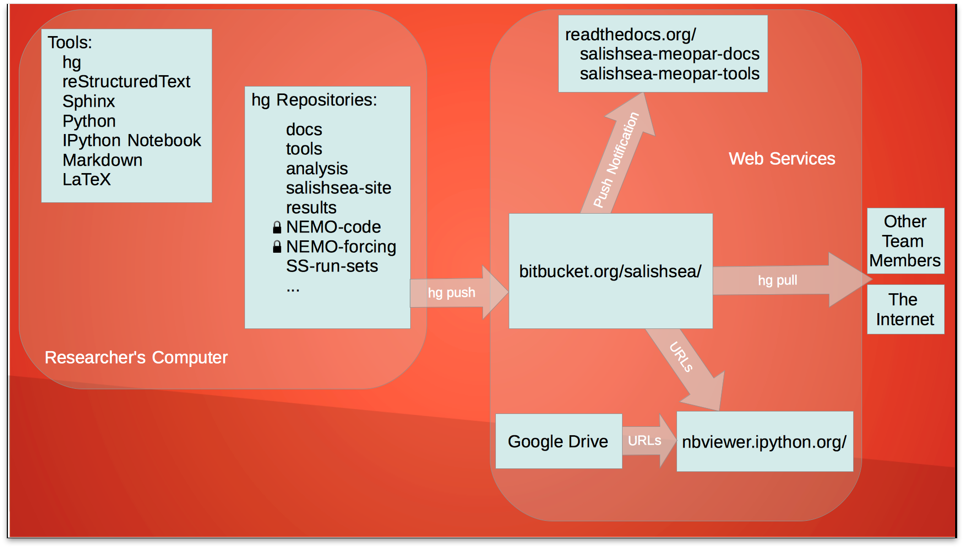
Collaboration via Distributed Version Control
What is Version Control (VC)?
Use software tools to keep a running record of 1 or more files.
Why You Should Use VC
- Lets you revert to earlier versions of your work
- Provides a record of what changed when
- Lets you mark significant points in time
- Allows you to play "what-if?"
- Facilitiates organized collaboration
- with your future self, as well as with other people
- Sync files among computers; laptop to desktop, desktop to HPC, ...
- "Provenance and change tracking are key to the scientific method; version control is the best actual way to do it" - Titus Brown
What You Should Use VC For
- Model Code
- Matlab/IDL/Python/R Scripts
- Plotting Scripts
- Processed Data Files & Scripts That Made Them
- Thesis
- Papers
- Reports
- ToDo List
Key Concept
Data differencing
Unix
diffandpatchutilitiesGiven a file, and a complete set of diffs between one state and another, any intermediate state for which there is a diff can be reconstructed.

Version Control Tools
Ad hoc:

Version Control Tools
http://en.wikipedia.org/wiki/Revision_control
Ad hoc:
thesis2.tex, JFM-21mar.doc, pooh.txt, ...
Mists of time...
- SCCS
- RCS
Proprietary:
- Visual SourceSafe
- Perforce
- BitKeeper
Version Control Tools
http://en.wikipedia.org/wiki/Revision_control
Old School (Client/Server):
- CVS (Concurrent Version System)
- SVN (Subversion)
Distributed & Open Source:
- GNU arch
- Darcs
- Monotone
Bazaar
Git
Mercurial
Pros and Cons
Ad hoc
- Easy to do, if you think of it
- Works best if you have a system
stuff1.txt,stuff2.f90,stuff4.mprobably isn't a good enough system- Hard to provide your future self with enough metadata
Client/Server
- Good for centrally controlled project; e.g. NEMO, ROMS, ...
- Work required to set up and administer
- Committing changes feels like a big deal
- Requires network connection
Distributed
- Almost zero set up
- No network required
- Every copy of a repository is a full backup
- Scalable to big projects
- Usable for central control
Git - A Quick Tour
http://git-scm.com/documentation
Pro Git book: http://git-scm.com/book
$ git help
Git Commands to Start a Project
$ git init myproject
$ cd myproject
add/create some files
$ git add
$ git commit -m"Initial commit."
Key Disciplines
Commit Early, Commit Often
- Small incremental changes are easier to understand
- You can't revert to a diff that doesn't exist
Make Commit Messages Informative
- 1st line is a summary; sometimes that's all you need
- Add more details in subsequent paragraphs
- Use present tense; e.g. "Fix typos."
- See http://tbaggery.com/2008/04/19/a-note-about-git-commit-messages.html
git Commands to See What's Going On
Print revision history of files or whole repository:
$ git log
Show differences between revisions:
$ git diff
Show status of files (e.g. modified, added, removed, missing, not tracked)
$ git status
N.B. There are lots of options for each command. See git help command
Tags
Tags are symbolic names for specific revisions in the repository. Most often you assign a tag to the current revision (HEAD) to mark a significant event.
Tag the current revision as jgr_1:
$ git tag --anotate -m"1st submission to JGR." jgr_1
Print a list of the tags in the repository:
$ git tag --list
Git Commands to Work in a Shared Project
$ git clone project_repo
$ cd project
edit some files
$ git add file1 file2 file3
$ git commit -m"My changes."
$ git push
project_repo can be a path, or a URL (http, https, ssh)
Collaboration
- User to user
- Shared repos on a private or public server
- Web services like Bitbucket or GitHub
Bitbucket and GitHub
- Mercurial or Git
- Free unlimited public repos
- Free private repos with 5-8 collaborators; unlimited with educational identity
- Per-repo issue trackers, wikis
- Forking, pull requests
- GUI clients
- Getting started: Bitbucket 101
- Git only
- Free unlimited public repos
- Monthly fee for private repos; maybe reduces with educational identity
- Per-repo issue trackers, wikis
- Forking, pull requests
- GUI clients
- More buzz in open source communities
- Getting started: GitHub Bootcamp
Part 2 - Python Tools and Glue
- Python
- The scientific Python stack
Python as Glue
- Command Processors for the SOG 1-D and Salish Sea NEMO models
- Code repo maintenance tool for NEMO codebase
- Automated testing of SOG 1-D model
- Packages of functions to re-use and shared use
- Running the SOG 1-D model in real-time forecast mode - SoG-bloomcast
Python
- http://python.org
- Created in 1989 by Guido van Rossum
- Clear, readable syntax
- General purpose language
- Well documented, free, and cross-platform
- Expressive
- Dynamic execution
- Very high level, dynamic data types
- Extensive standard library, and ecosystem of 3rd-party packages
- Easily extended in C and C++
Python for Science & Engineering
- http://scipy.org
- NumPy - N-dimensional arrays
- SciPy - Library of fundamental scientific algorithms (in many cases just Python wrappers around time-tested Fortran and C implementations)
- Matplotlib - 2D plotting
- IPython Notebook - enhanced Python shell in the browser with rich text, math notation, inline plots, ...
- Pandas - Statistical data analysis and modeling
- The list goes on...
- Curated distributions:
- Anaconda from Continuum Analytics
- Canopy from Enthought
The Rubicon for Python in Science
- Curated distributions - Anaconda
- Expanded and Improved Documentation for NumPy, SciPy, and friends
- IPython Notebook
Python as Glue - Command Processors for Models
- Python has several command line tool frameworks
SOG 1-D Coupled Physics-Biogeochemical Model
Based on the argparse standard library module
SOG run- Runs model from 1 or more parameter value filesSOG batch- Execute a series of runs, possibly concurrently
Salish Sea NEMO 3-D Model
Based on the cliff command line tool package
salishsea run tides.yaml iodef.xml ../results/tides3
- Evolved from:
-
salishsea prepare- Create a NEMO run directory containing files and symlinks -
salishsea combine- Combine per-processor netCDF results files; optionally compress -
salishsea gather-combine+ move run inputs, outputs & metadata to results directory
salishsea get_cgrfmanages CGRF atmospheric forcing file collection
Marlin - NEMO Code Repo Maintenance
- Operates on a repo that is both a Mercurial repo and a SVN checkout of NEMO
- Automates pulling SVN updates 1 by 1 and commits them to Mercurial
- Merging local changes and testing done manually (for now...)
Automated Testing of SOG 1-D Model
- Buildbot continuous integration tool
- Manager process:
- Listens for changes pushed to SOG code repo
- Has schedule of weekly tests
- Worker processes:
- 11 test cases distributed over 7 workstations
- Web interface for status and on-demand test runs
- Email notification of test failures
Packages of Functions to Re-use and Share
Python Packaging Tools
- Aggregate functions, class definitions, etc. in modules
- Collect modules in packages
- Namespaces
- Manage dependencies
SalishSeaTools Package
bathy_tools- Viewing and manipulation of netCDF bathymetry filesnc_tools- Exploring and managing the attributes of netCDF filestidetools- Analysis and plotting tidal harmonics results from NEMOstormtools- Analysis of storm surge results from the Salish Sea Modelviz_tools- Functions to do routine tasks associated with plotting and visualizationhg_commands- API for Mercurial commands that other tools usenamelist- Parse Fortran namelist files as Python dictionary data structures- Publicly available in the https://bitbucket.org/salishsea/tools repo
Documentation at http://salishsea-meopar-tools.readthedocs.org/en/latest/SalishSeaTools/salishsea-tools.html
SoG-Bloomcast - SOG 1-D Model Real-time Forecast
Daily, quasi-operational forecast of the 1st spring phytoplankton bloom in the Strait of Georgia:
- Get near real-time forcing data from web services
- wind, weather, river flows
- Process forcing data into format for model input
- Run the SOG model 3 (or 30+) times concurrently
- Analyze the run results to calculate the forecast bloom date as well as early and late bounds
- Create time series and depth profile plots
- Render a results commentary and the plots as an HTML page via a template
- Push the HTML page to a web site
Do all of that while we get on with other research!
SoG-Bloomcast - SOG 1-D Model Real-time Forecast
- Get near real-time forcing data from web services
- wind, weather, river flows
Requests - HTTP for Humans
import requests

url = 'http://climate.weather.gc.ca/climateData/bulkdata_e.html'
params = {
    'stationID': 6831,
    'format': 'xml',
    'Year': 2014,
    'Month': 6,
    'Day': 1,
    'timeframe': 1,
}
response = requests.get(url, params=params)

print(response.text[:1000])
Requests - With Session Data
with requests.session() as s:
    s.post(disclaimer_url, data='I Agree')
    time.sleep(5)
    response = s.get(data_url, params=params)
SoG-Bloomcast - SOG 1-D Model Real-time Forecast
- Get near real-time forcing data from web services
- wind, weather, river flows
- Process forcing data into format for model input
Data Processing & Transformation
- XML
- Python standard library: xml.etree.ElementTree
- lxml (if you need to do lots, and do it faster)
- HTML (web scraping)
- CSV
- netCDF
- GIS
SoG-Bloomcast - SOG 1-D Model Real-time Forecast
- Get near real-time forcing data from web services
- wind, weather, river flows
- Process forcing data into format for model input
- Run the SOG model 3 (or 30+) times concurrently
Subprocess Module
import subprocess

cmd = 'nice -n 19 SOG < infile > outfile 2>&1'

proc = subprocess.Proc(cmd, shell=True)

while True:
   if proc.poll() is None:
     time.sleep(30)
   else:
     print('Done!)
     break
SoG-Bloomcast - SOG 1-D Model Real-time Forecast
- Get near real-time forcing data from web services
- wind, weather, river flows
- Process forcing data into format for model input
- Run the SOG model 3 (or 30+) times concurrently
- Analyze the run results to calculate the forecast bloom date as well as early and late bounds
- Create time series and depth profile plots
Matplotlib
import matplotlib.pyplot as plt

fig, ax_left = matplotlib.pyplot.subplots(1, 1)
ax_right = ax_left.twinx()

ax_left.plot(nitrate.time, nitrate.values, color='blue')
ax_right.plot(diatoms.time, diatoms.values, color='green')

ax_left.set_ytitle('Nitrate Concentration [uM N]')
ax_right.set_ytitle('Diatom Biomass [uM N]')
ax_left.set_xtitle('Year Day in 2014')

fig.savefig('nitrate_diatoms_timeseries.svg')

SoG-Bloomcast - SOG 1-D Model Real-time Forecast
- Get near real-time forcing data from web services
- wind, weather, river flows
- Process forcing data into format for model input
- Run the SOG model 3 (or 30+) times concurrently
- Analyze the run results to calculate the forecast bloom date as well as early and late bounds
- Create time series and depth profile plots
- Render a results commentary and the plots as an HTML page via a template
String Interpolation & Templating
page_tmpl = """
<h1>Strait of Georgia Spring Bloom Prediction</h1>
<p>
The median bloom date calculate from a
{member_count} ensemble forecast is
{bloom_dates['median']:%Y-%m-%d}
...
</p>
"""

page = page_tmpl.format(
   member_count=len(members),
   bloom_dates=bloom_dates,
   ...
)

with open('page.html', 'rt') as f:
   f.write(page)
SoG-Bloomcast - SOG 1-D Model Real-time Forecast
- Get near real-time forcing data from web services
- wind, weather, river flows
- Process forcing data into format for model input
- Run the SOG model 3 (or 30+) times concurrently
- Analyze the run results to calculate the forecast bloom date as well as early and late bounds
- Create time series and depth profile plots
- Render a results commentary and the plots as an HTML page via a template
- Push the HTML page to a web site
Subprocess (again)
rsync, scp, sftp, hg, git, ...
cmd = [
    'rsync',
    '-Rtvhz',
    '{}/./{}'.format(html_path, results_page),
    'shelob:/www/salishsea/data/'
]
subprocess.check_call(cmd)
SoG-Bloomcast - SOG 1-D Model Real-time Forecast
Daily, quasi-operational forecast of the 1st spring phytoplankton bloom in the Strait of Georgia:
- Get near real-time forcing data from web services
- wind, weather, river flows
- Process forcing data into format for model input
- Run the SOG model 3 (or 30+) times concurrently
- Analyze the run results to calculate the forecast bloom date as well as early and late bounds
- Create time series and depth profile plots
- Render a results commentary and the plots as an HTML page via a template
- Push the HTML page to a web site
Do all of that while we get on with other research!
Shell Script and Cron Job
Shell script to run SoG-bloomcast:
# cron script to run SoG-bloomcast
#
# make sure that this file has mode 744
# and that MAILTO is set in crontab
VENV=/data/dlatorne/.virtualenvs/bloomcast
RUN_DIR=/data/dlatorne/SOG-projects/SoG-bloomcast/run
. $VENV/bin/activate && cd $RUN_DIR && $VENV/bin/bloomcast config.yaml
Cron entry to trigger the script daily:
MAILTO=dlatornell@eos.ubc.ca

BLOOMCAST_DIR=/data/dlatorne/SOG-projects/SoG-bloomcast
# m h  dom mon dow   command
  0 9   *   *   *    $BLOOMCAST_DIR/cronjob.sh
Python Tools and Glue
- Command Processors for the SOG 1-D and Salish Sea NEMO models
- Code repo maintenance tool for NEMO codebase
- Automated testing of SOG 1-D model
- Packages of functions to re-use and shared use
-
Daily, quasi-operational forecast of the 1st spring phytoplankton bloom in the Strait of Georgia:
- Get near real-time forcing data from web services
- wind, weather, river flows
- Process forcing data into format for model input
- Run the SOG model 3 (or 30+) times concurrently
- Analyze the run results to calculate the forecast bloom date as well as early and late bounds
- Create time series and depth profile plots
- Render a results commentary and the plots as an HTML page via a template
- Push the HTML page to a web site
Do all of that while we get on with other research!
Part 3 - Visualization of Model Results
In support of the Salish Sea NEMO project we are developing a collection of IPython Notebooks that provide discussion, examples, and best practices for plotting various kinds of model results from netCDF files. They include:
- Plotting code examples
- Examples of the use of functions from the
salishsea_toolspackage
The notebooks so far:
- Exploring netCDF Files.ipynb
- Plotting Bathymetry Colour Meshes.ipynb
- Plotting Tracers on Horizontal Planes.ipynb
- Plotting Velocity Fields on Horizontal Planes.ipynb
The links are to static renderings of the notebooks provided by the nbviewer.ipython.org service.
The notebook sources are in the analysis_tools directory of the public https://bitbucket.org/salishsea/tools/ repo.